Jeffreys centroid/Symmetric Kullback-Leibler centroid

This page provides you some basic R code implementing the algorithms described in:
Jeffreys Centroids: A Closed-Form Expression for Positive Histograms and a Guaranteed Tight Approximation for Frequency Histograms (opens in new tab)
It allows you to compute the centroid (or barycenter) with respect to the Jeffreys divergence:

also called symmetric Kullback-Leibler divergence (SKL, symmetrized Kullback-Leibler divergence).
Those frequency/positive Jeffreys centroids are defined as follows:

Scroll to the end to get the slides explaining the method.

Once we get a centroid, you can use center-based clustering techniques like k-means (Lloyd batched updates or Hartigan single swap update). Note that the center relocation in k-means need not be the optimal centroid but only improves over the current center: This is called variational k-means and applies to the Jeffreys frequency approximation technique.

Histograms

Consider the two renown images: barbara and lena (in grey color, PNG image format).


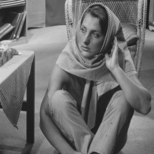
Barbara	Lena

We compute the (grey) intensity frequency histograms: We first compute the number of pixels having grey values g for g=0...255, add 1 to empty bins and renormalize so that the cumulative sum adds up to one.
You get the following frequency histograms (stored in ASCII format):

For Lena.histogram the file begins with:

3.8109756E-6
3.8109756E-6
3.8109756E-6
4.5731707E-5
2.5152438E-4
4.2682927E-4
6.2881096E-4
9.984756E-4
0.0011775915
0.0016463414
0.0020503048
0.0026028964
0.0032278963
...

Calculating centroids in R

Let us use the R language. Create a working directory C:\testR and put in that directory the files Lena.histogram and Barbara.histogram Then let us set this directory as the working directory in R (type in the R console):

setwd("C:/testR")

We load the histograms as follows:

lenah=read.table("Lena.histogram")
barbarah=read.table("Barbara.histogram")

You can print the histogram of lena simply by typing in the R console:

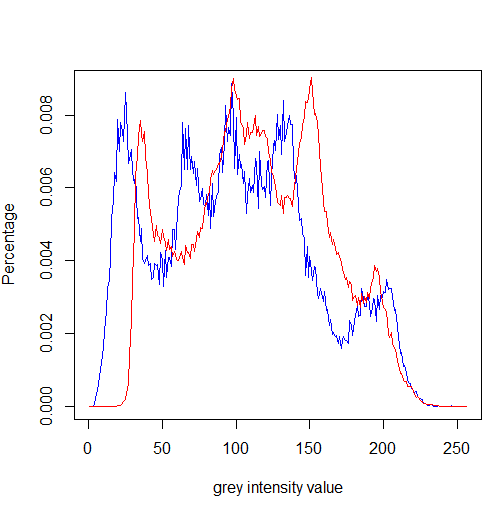
lenah

Let us visualize the frequency histograms:

plot(lenah[,1], type="l", col = "blue", xlab="grey intensity value", ylab="Percentage")
lines(barbara[,1], type="l",col = "red" )

Let us now source the R script file JeffreysSKLCentroid.R (download and put this file in the working directory, you can also view the code below):

source("JeffreysSKLCentroid.R")

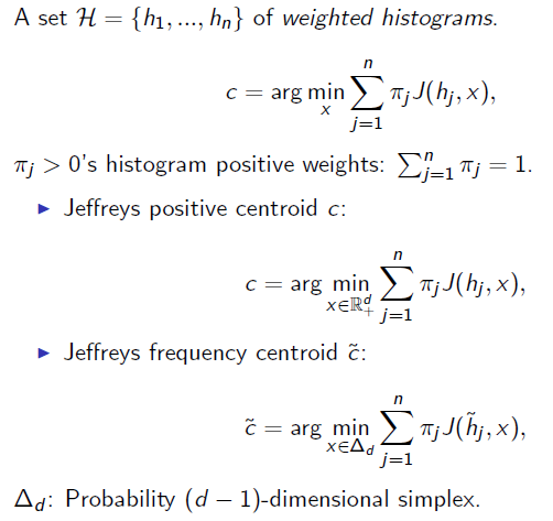
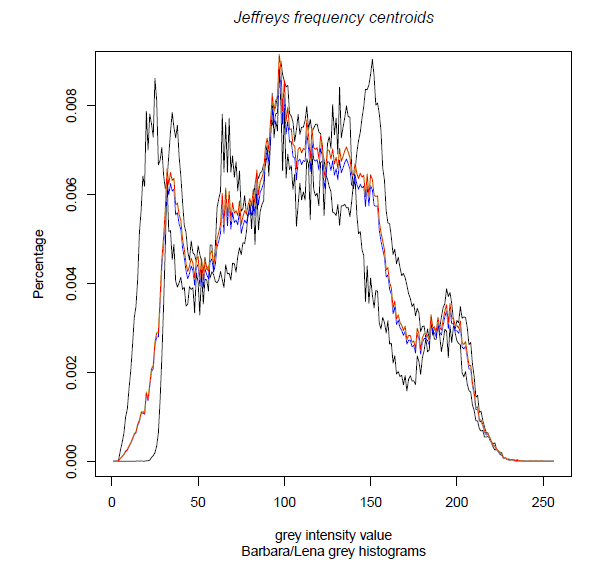
To compute the following centroids:

approxP: Jeffreys optimal positive centroid (almost but not optimal frequency centroid!),
approxF Jeffreys frequency centroid approximation by renormalizing approxP (almost but not frequency!),
approxFG: Jeffreys optimal frequency centroid (up to machine precision using an interative algorithm),

let us execute this code:

n<-2
d<-256
weight=c(0.5,0.5)
set<- array(0, dim=c(n,d))
set[1,]=lenah[,1]
set[2,]=barbarah[,1]
approxP=JeffreysPositiveCentroid(set,weight)
approxF=JeffreysFrequencyCentroidApproximation(set,weight)
approxFG=JeffreysFrequencyCentroid(set,weight)

We can now visualize the three centroids:

pdf(file="SKLJeffreys-BarbaraLena.pdf", paper ="A4")
typedraw="l"
plot(set[1,], type=typedraw, col = "black", xlab="grey intensity value", ylab="Percentage")
lines(set[2,], type=typedraw,col = "black" )
lines(approxP,type=typedraw, col="blue")
# green not visible, almost coincide with red
lines(approxF, type=typedraw,col = "green")
lines(approxFG,type=typedraw, col="red")
title(main="Jeffreys frequency centroids", sub="Barbara/Lena grey histograms" , col.main="black", font.main=3)
dev.off()
graphics.off()

You can download the full R console session:SessionJeffreysR.txt. Copy/paste in the R console and inspect the pdf file SKLJeffreys-BarbaraLena.pdf. Let us now draw randomly some sets of frequency histograms and compute their Jeffreys centroids:


randomUnitHistogram<-function(d)
{
result=runif(d,0,1); 
result=result/(cumsum(result)[d]) 
result
}

n<-10  # number of frequency histograms
d<-25  # number of bins
set<- array(0, dim=c(n,d))
weight<-runif(n,0,1); 
cumulw<-cumsum(weight)[n]

# Draw a random set of frequency histograms
for (i in 1:n)
{set[i,]=randomUnitHistogram(d)
weight[i]=weight[i]/cumulw;
}

A=ArithmeticCenter(set,weight)
G=GeometricCenter(set,weight)
nA=normalizeHistogram(A) # already normalized 
nG=normalizeHistogram(G)
# Simple approximation (half of normalized geometric and arithmetic mean)
nApproxAG=0.5*(nA+nG)

optimalP=JeffreysPositiveCentroid(set,weight) 
approxF=JeffreysFrequencyCentroidApproximation(set,weight)
# guaranteed approximation factor
AFapprox=1/cumulativeSum(optimalP);

# up to machine precision
approxFG=JeffreysFrequencyCentroid(set,weight)

Finally, let us output graphically those centroids into a pdf file:

pdf(file="SKLJeffreys-ManyHistograms.pdf", paper ="A4")
typedraw="l"
plot(set[1,], type=typedraw, col = "black", xlab="grey intensity value", ylab="Percentage")
for(i in 2:n) {lines(set[i,], type=typedraw,col = "black" )}
lines(approxFG,type=typedraw, col="blue")
lines(approxF, type=typedraw,col = "green")
lines(optimalP,type=typedraw, col="red")
title(main="Jeffreys frequency centroids", sub="many randomly sampled frequency histograms" , col.main="black", font.main=3)
dev.off()

Here is the result: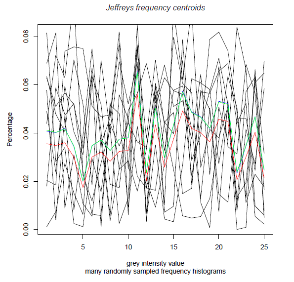

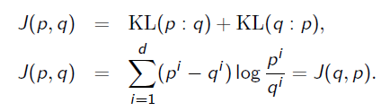
(snapshot of file SKLJeffreys-ManyHistograms.pdf)
Observe that the green/blue frequency histograms (Jeffreys normalized positive histogram, Jeffreys frequency histogram computed up to machine precision) almost coincide but are fairly different from the optimal Jeffreys positive centroid.

Slides

Slides in pdf (open in new tab).

Slides: Jeffreys centroids for a set of weighted histograms from Frank Nielsen

Link to Bregman symmetrized centroids

A frequency histogram may be interpreted as the parameter of a multinomial distribution (with fixed number of trials). The Kullback-Leibler divergence amounts to compute a Bregman divergence for exponential families. Therefore the Jeffreys divergence is equivalent (for exponential families) to a symmetrized Bregman divergence. Thus the SKL centroid (Jeffreys centroid) can be interpreted as a symmetrized Bregman centroid.

See:
Sided and symmetrized Bregman centroids. IEEE Transactions on Information Theory 55(6): 2882-2904 (2009)

Citation

Frank Nielsen: Jeffreys Centroids: A Closed-Form Expression for Positive Histograms and a Guaranteed Tight Approximation for Frequency Histograms. IEEE Signal Process. Lett. 20(7): 657-660 (2013)
BibTeX

@ARTICLE{JeffreysSKLCentroid-2013, 
author={Nielsen, Frank}, 
journal={IEEE Signal Processing Letters}, 
title={Jeffreys Centroids: A Closed-Form Expression for Positive Histograms and a Guaranteed Tight Approximation for Frequency Histograms}, 
year={2013}, 
volume={20}, 
number={7}, 
pages={657-660}, 
doi={10.1109/LSP.2013.2260538}, 
ISSN={1070-9908}
}

Some sanity check

In the paper, we show that:

Let us check this:

Lambda<-function(set,weight) 
{
na=normalizeHistogram(ArithmeticCenter(set,weight))
ng=normalizeHistogram(GeometricCenter(set,weight))
d=length(na)
bound=rep(0,d)
for(i in 1:d) {bound[i]=na[i]+log(ng[i])}
lmin=max(bound)-1 
lmax=0
while(lmax-lmin>1.0e-10)
{
lambda=(lmax+lmin)/2
cs=cumulativeCenterSum(na,ng,lambda);
if (cs>1)
{lmin=lambda} else {lmax=lambda}
}

lambda
}

JeffreysFrequencyCentroid<-function(set,weight) 
{
na=normalizeHistogram(ArithmeticCenter(set,weight))
ng=normalizeHistogram(GeometricCenter(set,weight))
lambda=Lambda(set,weight)
JeffreysFrequencyCenter(na,ng,lambda)
}


KullbackLeibler<-function(p,q)
{
d=length(p)
res=0
for(i in 1:d)
{res=res+p[i]*log(p[i]/q[i])+q[i]-p[i]}
res
}


lambda=Lambda(set,weight)
ct=JeffreysFrequencyCentroid(set,weight)
na=normalizeHistogram(ArithmeticCenter(set,weight))
ng=normalizeHistogram(GeometricCenter(set,weight))

# Check that $\lambda=-\KL(\tilde{c}:\tilde{g})$
lambdap=-KullbackLeibler(ct,ng)
lambda
# difference
abs(lambdap-lambda)

We get the following console output which corroborates the lambda/KL identity:

> lambda
[1] -0.01237374696329113926696
> # difference
> abs(lambdap-lambda)
[1] 5.261388026644997495396e-11

Main code:JeffreysSKLCentroid.R


options(digits=22)
PRECISION=.Machine$double.xmin

LambertW0<-function(z)
	{
		S = 0.0
		for (n in 1:100)
		{
			 Se = S * exp(S)
			 S1e = Se + exp(S)  
			if (PRECISION > abs((z-Se)/S1e)) { 
			break}
			S = S -	(Se-z) / (S1e - (S+2) * (Se-z) / (2*S+2))
		}
		S
	}

#
# Symmetrized Kullback-Leibler divergence (same expression for positive arrays or unit arrays since the +q -p terms cancel)
# SKL divergence, symmetric Kullback-Leibler divergence, symmetrical Kullback-Leibler divergence, symmetrized KL, etc.
#
JeffreysDivergence<-function(p,q)
{
d=length(p)
res=0
for(i in 1:d)
{res=res+(p[i]-q[i])*log(p[i]/q[i])}
res
}

normalizeHistogram<-function(h)
{
d=length(h)
result=rep(0,d)
wnorm=cumsum(h)[d]
for(i in 1:d)
{result[i]=h[i]/wnorm; }
result
}

#
# Weighted arithmetic center 
#
ArithmeticCenter<-function(set,weight)
{
dd=dim(set)
n=dd[1]
d=dd[2]
result=rep(0,d)
for(j in 1:d)
{
for(i in 1:n)
{result[j]=result[j]+weight[i]*set[i,j]}
}
result
}

#
# Weighted geometric center
#
GeometricCenter<-function(set,weight)
{
dd=dim(set)
n=dd[1]
d=dd[2]
result=rep(1,d)
for(j in 1:d)
{
for(i in 1:n)
{result[j]=result[j]*(set[i,j]^(weight[i]))}
}
result
}

cumulativeSum<-function(h)
{
d=length(h)
cumsum(h)[d]
}

#
# Optimal Jeffreys (positive array) centroid expressed using Lambert W0 function 
#
JeffreysPositiveCentroid<-function(set,weight) 
{
dd=dim(set)
d=dd[2]
result=rep(0,d)
a=ArithmeticCenter(set,weight)
g=GeometricCenter(set,weight)
for(i in 1:d)
	{result[i]=a[i]/LambertW0(exp(1)*a[i]/g[i])}
result
}

#
# A 1/w approximation to the optimal Jeffreys frequency centroid (the 1/w is a very loose upper bound)
#
JeffreysFrequencyCentroidApproximation<-function(set,weight) 
{
result=JeffreysPositiveCentroid(set,weight) 
w=cumulativeSum(result)
result=result/w
result
}

#
# By introducing the Lagrangian function enforcing the frequency histogram constraint
#
cumulativeCenterSum<-function(na,ng,lambda)
{
d=length(na)
cumul=0
for(i in 1:d)
{cumul=cumul+(na[i]/LambertW0(exp(lambda+1)*na[i]/ng[i]))}
cumul
}

#
# Once lambda is known, we get the Jeffreys frequency cetroid
#
JeffreysFrequencyCenter<-function(na,ng,lambda)
{
d=length(na)
result=rep(0,d)
for(i in 1:d)
{result[i]=na[i]/LambertW0(exp(lambda+1)*na[i]/ng[i])}
result
}

#
# Approximating lambda up to some numerical precision for computing the Jeffreys frequency centroid 
#
JeffreysFrequencyCentroid<-function(set,weight) 
{
na=normalizeHistogram(ArithmeticCenter(set,weight))
ng=normalizeHistogram(GeometricCenter(set,weight))
d=length(na)
bound=rep(0,d)
for(i in 1:d) {bound[i]=na[i]+log(ng[i])}
lmin=max(bound)-1 
lmax=0
while(lmax-lmin>1.0e-10)
{
lambda=(lmax+lmin)/2
cs=cumulativeCenterSum(na,ng,lambda);
if (cs>1)
{lmin=lambda} else {lmax=lambda}
}

JeffreysFrequencyCenter(na,ng,lambda)
}